Principels of Damage Detection
The Observalibility Matrix
Common to all the damage detection techniques in the software is that they are based on the same principles as the Stochastic Subspace Identification (SSI) techniques. The crucial part of SSI is to decompose a Hankel matrix (coming from the measurements) using Singular Value Decomposition, then identify a subspace of the largest singular values, and from here estimate the so-called Observability matrix. The Observability matrix contains the information about the physical modes that SSI has been able to extract from the measurements with the given subspace of singular values.
In this paper of Döhler et al. the Observalility matrix is introduced in section 2.2.
Since the Observability matrix is constructed from manipulation of the measurements of the physical behavior of a structure, it is a matrix that describes the behavior of the structure in physical domain. No modal decomposition (eigenvalue decomposition) has taken place, which means that information of all excited modes between DC and the Nyquist frequency is in fact contained i the matrix.
Detection Strategy
In damage detection the aim is to compare the Observability matrix of a reference state with the same matrix obtained in a potential damage state. There are various ways to compare two matrices, but in the software this is done by the so-called Chi-Squares testing.
In principel, the two matrices are subtracted and the result is vectorized by stacking all the columns of resulting matrix to form a residual vector. This vector should basically only consist of zeroes, but there will always even small values present even though the two Observalibility matrices are obtained from the same (undamaged) system.
In practise, the residual of the two matrices are obtained by first estimating the left Null-space of the Hankel matrix obtained from the measurements of the reference state. Then the Hankel matrix, constructed from measurements of a potential damage state, is multiplied with this Null-space. In the software, the Reference State Validation window is used to validate this left Null-space.
So in order to test if the residual values are small enough to conclude that the two matrices are "the same" a statistical framework is needed. This is the Chi-Squares testing. The Chi-Squares testing of the residual vector need some statistics about the natural level of the residuals in the undamaged state. This statistics is represented by a covariance matrix of the residuals, which need to be estimated from a series of reference measurements.
Once the covariance matrix is estimated, then all the reference measurements can be tested, which will lead to a series of scalar Chi-Squares values. From these a threshold of the natural (undamaged) level of the Chi-Squares values can be determined. This threshold is basically estimated as the standard deviation of the Chi-Squares values multiplied with some significance level factor.
In the paper of Döhler et al. the Chi-Squares testing is introduced in section 2.3.
Classical and Robust Detection
In the software, there are two Damage Detection approaches: Classic and Robust. The Classic use the principles as described above and the Robust use a slight change of the above to compensate for potential changes in vibration levels across the different measurements.
In the paper of Döhler et al. the Robust approach is introduced in section 3.
In general both methods works in case of changing excitation levels. In case of the Classic a normalization of the channel standard deviations is used to account for such changes. However, for validation purposes, it is good to have several estimates available, and if a joint damage indicator is desired, this one can be obtained by switching to the Control Chart that can join several indicators into a single control value.
Damage Detection in Practise
The section below describes the various steps of the practical damage detection. The details are also given in this YouTube video Damage Detection.
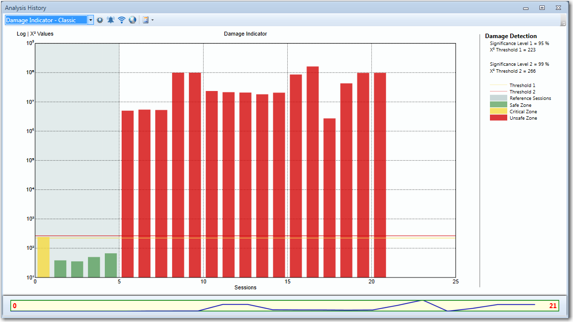
The outcome of the damage detection is a diagram like shown below. As long as the structures dynamic performance is the same the bars representing the Chi-Squares values are green. As the structure start to deterioate the residuals becomes significant larger resulting in a significant increase of the Chi-Square value. Now it will exceed the threshold(s) and the bar becomes red.
The Damage Detection Toolbar
The Damage Detection has the toolbar with the following options available:
 Configure and Start the Damage Detection.
 Configure the Notifications to be send out. For more info check out the Analysis History Notifications
 Send the E-mail and Web Service notifications manually i.e. On Demand
 Opens the default web browser if the web site Url is specified.
Damage Detection Configuration
Starting the Damage Detection Configuration will start up the dialog below:
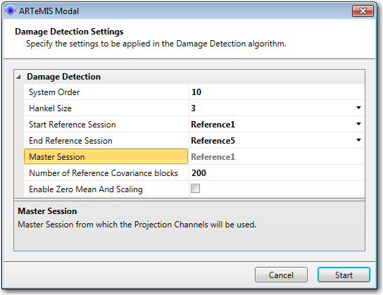
The following settings should be defined in order to get the optimal and correct results:
- System Order. This value should be set so that it divides the singular values in significant and insignificant ones. See Reference State Validation window.
- Hankel Size. Normally you should set this one to Auto to start. Once processing is finished, it will indicate the automatic selected size. Increase or decrease if needed. See Reference State Validation window.
- Reference Range (Start and End Reference). These two drop down lists allow you to select what sessions (measurements) to use for the construction of the Reference State Model. It is critical to have several sessions as this increase the robustness of the statistics of the Reference State Model. Do not include all available reference sessions, as it is a good idea to use some for validation of the performance of the Reference State Model. These unused reference session should not have Chi-Squares values that exceed the thresholds (become red). If this is the case, then the Reference State Model is inappropiate.
- Master Session (read only, defined through the Signal Processing Control in the Prepare Data task).
- Number of Reference Covariance blocks. Normally this is not a value that needs to be adjusted. It is the number of segment each sessions measurements are cutted into during the estimation of the residual covarnace matrix.
- Enable Zero Mean And Scaling. Check this one if there are significant changes of the vibration level of the different measurements (sessions).
Once the settings are specified, clicking on the Start button will close the dialog and start the Damage Detection analysis. If needed go back and reconfigure and start the analysis again. See Reference State Validation window for possible reasons to re-run the analysis.
Damage Detection Property Grid
Once the Damage Detection is calculated, additional settings can be specified through the Property Grid
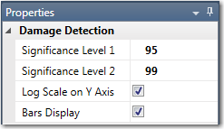
The Significance Levels define the level of the two available thresholds. When Level 1 is passed by a Chi-Squares value, then it leaves the Safe-Zone (undamaged) and enter the Critical Zone, which can be considered the first warning that something is changing. When it passed Level 2 then it enter the Unsafe-Zone (damaged). The levels of the threshold are given in terms of statistical significance levels. By default, Level 1 is the 95% probability that a significant change has happened. Level 2 is the 99% significance level. These can be changed if required.
Log Scale on Y Axis toggles if the Y axis is displayed in logarithmic scale. This may be required since the calculated values may be extremely large range.
Bars display toggles the display between a bar (chart) display and a continuous line display.
Control Chart
The Control Chart does not have a specific configuration. The Control chart Values depend on the Chi Square Values from the Damage Detection.
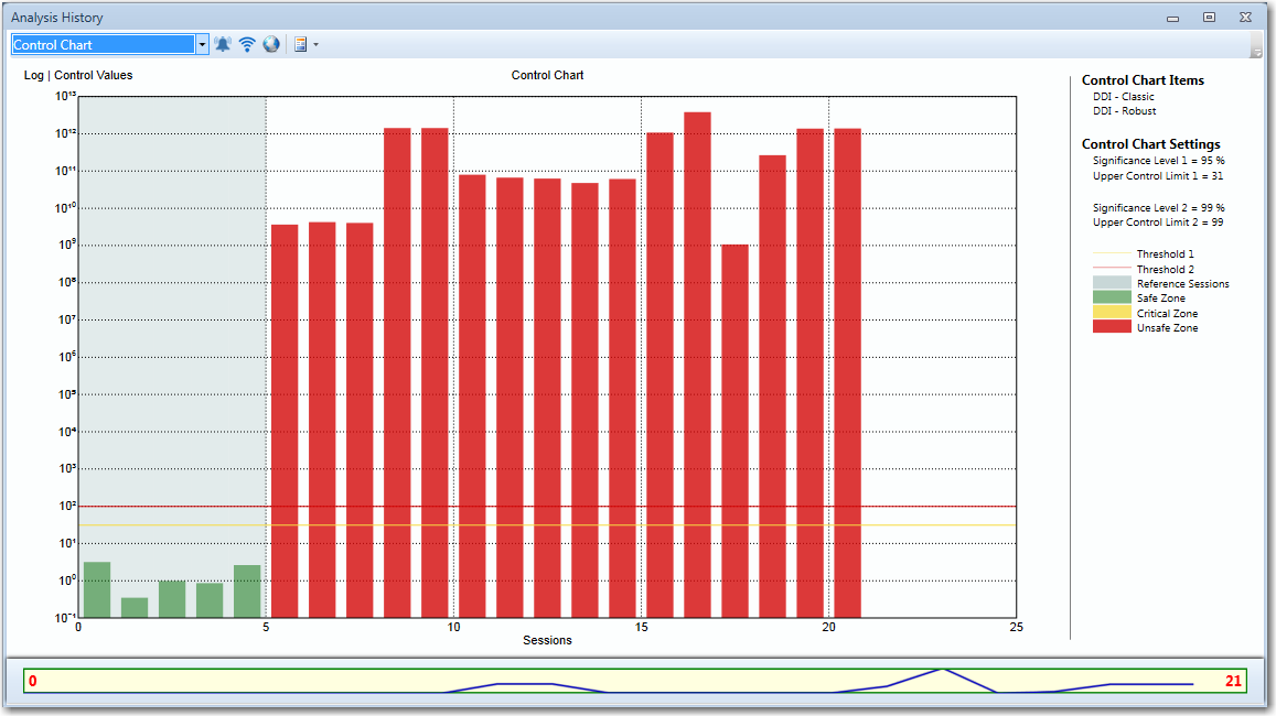
The Control Chart should include at least one of the two Damage Detection methods. This can be specified from the Property Grid Control Chart Items:
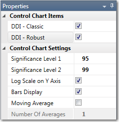
Additional Control Chart Settings are available to customize the Control Chart diagram:
The Significance Levels define the level of the two available thresholds. When Level 1 is passed by a Chi-Squares value, then it leaves the Safe-Zone (undamaged) and enter the Critical Zone, which can be considered the first warning that something is changing. When it passed Level 2 then it enter the Unsafe-Zone (damaged). The levels of the threshold are given in terms of statistical significance levels. By default, Level 1 is the 95% probability that a significant change has happened. Level 2 is the 99% significance level. These can be changed if required.
Log Scale on Y Axis toggles if the Y axis is displayed in logarithmic scale. This may be required since the calculated values may be extremely large range.
Bars display toggles the display between a bar (chart) display and a continuous line display.
Moving Average is used to perform a smoothing of the control values. This can be necessry in order to see how the trend is in case of noisy control values.
Number Of Averages indicate how many control values to average during the smoothing operation.